Exponential growth follows x(t) = x₀(1+r)^t, where the growth rate r = EP combines daily exposures E with the per-exposure infection probability P. Estimate r as the day-on-day ratio of confirmed cases. A real epidemic eventually bends into a logistic S-curve, but until it does, a tiny change in r — 1.1 vs 1.2 — turns six million projected cases into nearly eight hundred million.
The Johns Hopkins Whiting School of Engineering maintains a regularly updated GitHub repository of Covid-19 data. Taking the confirmed cases outside China, we can watch how the count changed as the virus spread worldwide. The classic function for exponential growth of x over time is:
where t is the time period and r is the growth rate.
What makes up the growth rate?
The growth rate has two elements: the average number of people an infected person is exposed to in one day (E), and the probability that each such exposure results in a new infection (P). Computing the growth rate EP is just the ratio between the number of confirmed cases on day t and the number on day t−1. Assemble a table of confirmed cases over time and you can compute a growth rate for each day.
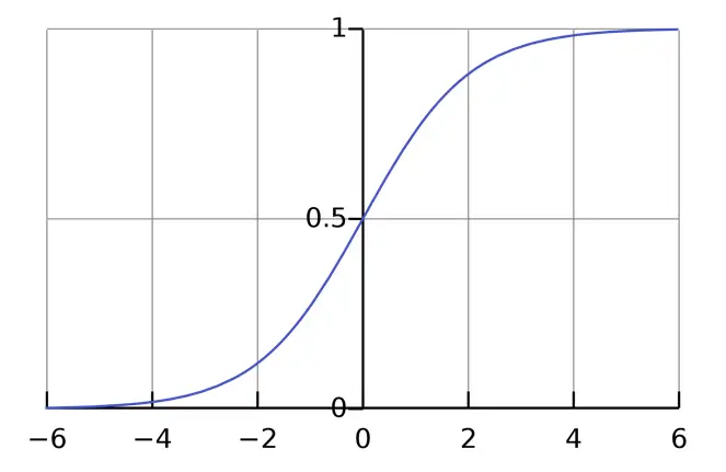
Where does exponential growth end?
Real growth doesn’t run forever — it follows a logistic, or S-shaped, curve that is near-exponential early on and then bends towards a ceiling. As a rule of thumb, the total number of infections ends up around twice the value at the inflection point. Plotting the growth rate for this early data, it sat around 1.2 with only a slight downward trend — suggesting some time still to go before it approached 1 (no further growth).
Why small changes matter so much
Knowing the growth rate lets us project forward, assuming it holds steady (and we can also model changes to E, P, or both). The table below projects confirmed cases outside China across several weeks and growth rates. It’s deliberately simplistic — it takes no account of world population or already-infected cases:
| Date | r = 1.1 | r = 1.15 | r = 1.2 |
|---|---|---|---|
| 1 week | 56,779 | 77,505 | 104,403 |
| 4 weeks | 420,184 | 1,458,762 | 4,803,079 |
| 8 weeks | 6,059,478 | 73,033,799 | 791,761,924 |
Even a small change in the growth rate elicits a dramatic change in the predicted number of cases — especially over time. That’s the deceptive power of an exponent.
Why this matters for energy
The same exponential intuition governs compounding loads, battery degradation, and demand growth on a constrained grid — small differences in rate compound into very different futures. It’s the reasoning behind the coming reliability gap and the structural-demand questions in data centres, AI and the grid.